结果部分是一般性的陈述，解释从实验测量中获得的原始数据。结果部分是论文的核心，是研究工作最重要的部分。所有其他部分都是次要角色，（它们）要么是为读者准备结果，要么是为增加的发现提供补充信息。

结果部分以文本、插图和表格的形式体现出来。三种形式都可以使用，但同样的数据不能在多种格式里重复使用。

结果部分的文本可以是任何长度。有时可以像一个陈述那样简洁。“结果见图1-4和表Ⅰ-Ⅲ”，这就足矣。为了清楚起见，文本中的长段落通常可以通过主题分成几个小部分，然后再为每个主题设立副标题，从而帮助读者寻找自己感兴趣的段落。

有时“结果”和“讨论”部分被组合成一个大部分，尤其是当原始数据必须被讨论以解释为什么采用后续的数据时。

不管采取什么格式，都应该遵循以下的原则：

1.只强调那些重要的实验观察，这些观察能够回答或解决在引言中提到的问题。

2.结果要有选择性。过多的细节对读者会是个负担，甚至可能会使读者糊涂，令其失去兴趣。细节数据应放置在补充材料部分（经常用小字体印刷，出现在论文末尾），或者属于论文之外的数据库。

3.组织好文本，以便强调结果。对于有关材料和方法的辅助信息，图片中的图例、表格的标题等，不要强调太多。它们可以通过书写技巧来实现，比如把表述结果的句子放在段首，把辅助信息放在从句中，或者使用被动语态。例如：

We broke the disulfide bonds of ribonuclease A by dithioerythreitol.This reduction denatured the proteins.

上面的例子首先描述实验步骤，然后用一个独立的句子来表述结果（蛋白质的变性）。这一次序强调的重点是程序而不是结果。此外，主动语态的使用重点强调的是主语“我们”而不是“二硫键”（disulfide bonds）。尽管主动语态常常在写作中受到偏爱，但在这个例子中，它却强调了错误的要素。句子可以修改为：

When the disulfide bonds of ribonuclease A were broken with dithioerythreitol，the reduced protein was denatured.

在此句中，方法在从句中被描述，而结果作为句子的主体得到更多强调。句子还可以修改为：

The breaking of the disulfide bonds of ribonuclease A by dithioerythreitol denatured the protein.

或

Ribonuclease A was denatured by breaking its disulfide bonds with dithioerythreitol.（假定读者已经知道二硫苏糖醇对于二硫键来说是一种还原剂。）

综上所述，若想对实验结果加以强调，一个行之有效的方法就是在首句陈述总结结果，在接下来的句子中，提供辅助细节。例如：

The conformation of Phaseolus caralla lectin was stable between pH4 and 10.The protein was denatured at pH12，but its conformation could be restored upon lowering the alkaline pH to neutral.However，denaturation at pH13 was irreversible.

4.不要把可能属于论文其他部分，如“材料和方法”部分的信息包含进来。

5.不要在文本中重复图片中的图例或者表格的标题。

6.在文本中只解释那些对读者来说难以理解的插图、表格所体现的重要信息，或插图和图表中显而易见的重要特征。

例1

Based on circular dichroic spectra，the conformation of lysozyme was completely unordered above 70℃（fig.l）.

or

Circular dichroic spectra（fig.l.）indicated that lysozyme was thermally denatured above 70℃.

例2

The binding of oxygen to hemoglobin increased with increasing pressure of oxygen（Table 1）.

而不是简单重复插图和表格中提供的数据。

例3

Figure 1 shows the conformation of lysozyme as a function of temperatures.The circular dichroic spectra indicated that the protein was completely unfolded above 70℃.

例4

Table 1 lists the percent binding of Oxygen to hemoglobin as a function of the oxygen pressure.It increased with increasing pressure of oxygen.

7.一定要确保文本、插图和表格互相保持一致。这一点看起来显而易见，但是我们经常发现表格中的数值与插图不一致，或者表格和图形中的数据在文本中被错误地引用。

8.如果合适的话，运用统计的方法分析你的数据。

9.不要省略那些不支持你的假设和结论，或者没有回答研究问题的数据。

10.在结果部分常用过去时态，除非涉及图片和表格。当涉及图片和表格时，常用现在时。如：

①Tacrine inhibited the activity of acetylcholinesterase noncompetitively.

②The data in Table 1 were collected over a four-month period.

③Table 1 contains data collected over a four-month period.

11.句首为术语时，读起来比较费劲。一个句子不应该把一个简化的术语放在句首，除非这个术语有广为约定俗成的缩写形式。如下列句子：

①Fig.1 shows...

②Deoxyribonucleic acid tests are used in forensic laboratories.

③Doctor Kevin Anderson performed the tests.

应该对应地改为：

①Figure 1 shows...

②DNA tests are used in forensic laboratories.

③Dr.Kevin Anderson performed the tests

例②和例③中，DNA和Dr.的用法远远超过他们本身的全称用法。

12.数据和符号不应该放在句首。以数据或符号开始一个句子，拼出来较吃力，句子应该重写。如下列句子：(www.daowen.com)

①12 subjects were tested.

②1g of compound A was used.

③α-tocopherol was applied.

④1990 was the first year the conference was held.

应该对应地改为：

①Twelve subjects were tested.

②One gram of compound A was used.（Note that gram is also spelled out.）

③Alpha-tocopherol was applied.

④The conference was first held in 1990.

13.句子中的数字不应该以一个代数点开始。小于1的代数部分应该在小数点前加上数字0。例如：

.476，-.05

应改为：

0.476，-0.05

例：

3 Results

3.1.Ψsoiland θ observations

In all plots irrigation was initiated approximately one month after the start of the observation period.During the observation periods irrigation events alternated with periods of rainfall（Fig.4）.Although observed in different years，Ψsoilobservations in plot A（Fig.4a）and plot B（Fig.4b）were quite similar.Ψsoilon the irrigated side of the three（positions 1，2 and 3）decreased to-30 kPa while on the non irrigated side（positions 4，5 and 6）Ψsoildecreased to-50 kPa.Ψsoilincreased rapidly to 0 kPa when irrigation was applied.In the non irrigated C plot Ψsoildepleted to-70 kPa on position 2 and to-120 kPa on position 1（Fig.4c）.

Observations of θ were correlated with the Ψsoilobservations.R2 between θ sampled in the soil layer 0-30 cm and observed soil was 0.80，R2between θ sampled in the Ψsoillayer 30-60 cm and observedΨsoilwas 0.45.

3.2.Root distribution

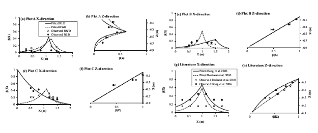
Coarse roots of the tree excavated in plot A rooted to a depth of 70 cm and reached the borders of the weed free strip beneath the canopy（Fig.5）.Fine roots were observed to a depth of 90 cm as presented in the relative root distributions（Fig.6a and b）.Maximal fine root density in plot A was observed at a depth of 22.5 cm while in other plots maximal fine root density was observed just beneath the soil surface（Fig.6c，d，e，f）.Maximal fine root density was not always observed close to tree.RLD was for plot B and C higher at 35 cm and 50 cm from the trunk.In plot A there was a good correspondence between RLD and RWD，R2 between both was 0.52.In plot B and plot C accordance was only moderate with R2 being 0.20 and 0.19 respectively.Root distributions derived from literature showed the highest RLD close to the tree（Fig.6g）.Distribution in the Z-direction was similar to the observations in plot B and C（Fig.6h）.

It was possible to fit the root distribution functionβ（x，z），suggested by Vrugt et al.（2001a）Eq.（7），through the fine root observations（Table 2）.For all plots the quality of the fit was satisfying with R2 0.70 or higher.Only for plots A and C the R2 of the fit through the observed RLD was lower in the X-direction.In the Z-direction R2 between the fit and the observations was higher than 0.73 for all plots.

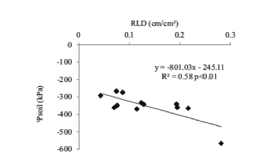
An interesting relation was observed betweenΨsoilrecorded on 15/05/2011 in plot B and C and the corresponding RLD（Fig.7）.Between the start of the observation period and 15/05/2011 no irrigation was executed yet and rainfall was limited so that the observed variation in Ψsoilreflects the water uptake pattern of the trees.No similar correlation could be observed between Ψsoiland RWD.

Fig.6.Root distributions β（x，z）used in the HYDRUS calculations.β（x，z）was fitted using the equations suggested by Vrugt et al.（2001a，b）through RLD and RWD observations in plot A（a，b），plot B（c，d），plot C（e，f）and through RLD observations reported in literature（g，h）.Parameters of β（x，z）according to Vrugt et al.（2001a，b）are presented in Table 2.

Fig.7.Relation between Ψsoilrecorded with the watermark sensors on 15/05/2011 in plot B，C and RLD on the same position.

Table 2.Parameters that define the root distributions β（x，z）used in the HYDRUS calculations according to Vrugt et al.（2001a，b）.Xm，Zmmaximum rooting depths in the X-and Z-direction，x and z are distances from the origin in the X-and Z-direction.Px，Pz，r*and z*are empirical parameters，R2:Pearson correlation coefficient between observed and fitted β（x，z）.β（x，z）is plotted in Fig.6.

3.3.Numerical calculations with HYDR US

The numerical calculation of Ψsoilcorresponded reasonable with the Ψsoil observations（Table 3）.However in the non-irrigated plot C a satisfying calculation of Ψsoilwas only possible whenβ（x，z）was based on RLD.Calculation of Ψsoilwithβ（x，z）based on RWD or root distributions found in literature yielded large errors.In plot A and B the calculation of Ψsoilwas only slightly better whenβ（x，z）was based on RLD compared to RWD or observations derived from literature.

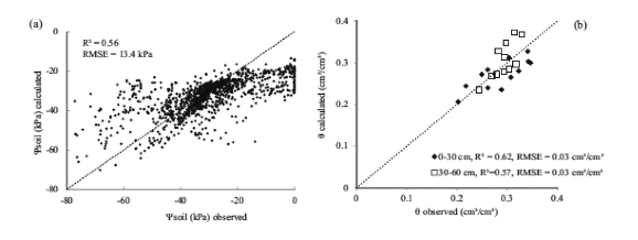
Overall correlation between all Ψsoilobservations and the corresponding Ψsoilcalculations was 0.56，RMSE was 13.40 kPa（Fig.8a）whenβ（x，z）was parameterized with RLD.Accordance between calculated and observed Ψsoil was erratic when observed Ψsoilranged between-20 kPa and 0 kPa.Ψsoil observed by the Watermark sensor was in this range always higher compared to Ψsoilachieved by the numerical calculation.Observations ofθ　agreed likewise with the calculated θ（Fig.8b），at the depth of 30-60 cm R2 was slightly lower compared to 0-30 cm depth.

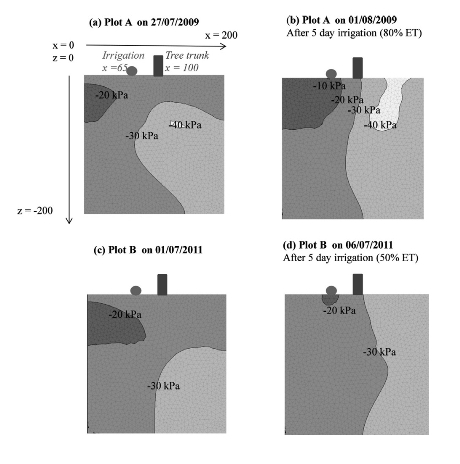
The numerical calculation showed how water was distributed in the root zone after irrigation.After a 80%ET irrigation periodin plot A Ψsoil increased above-20kPa in the entire irrigated side of the tree to a depth of 70 cm（Fig.9a and b）.By applying 50%ET irrigation in plot B Ψsoilincreased to-20 kPa only at a distance of 15 cm from the dripper（Fig.9c and d）.

Table 3 Quality of the HYDRUS calculation in each plot quantified by the R2 between observation and simulation and the RMSE expressed in kPa.The numerical calculation of Ψsoilby HYDRUS was based on root distributions parameterized with Root Length Density（RLD），Root Weight Density（RWD）and root observations described in literature（Gong et al.，2006，Besharat et al.，2010）.

Fig.8.Agreement between all（n=1320）Ψsoilobservations（a）and all（n=24）θ observations（b）and the corresponding numerical calculations ofΨ soilandθ .Root distributions of the numerical calculations were based on RLD.

Fig.9.Output of the Ψsoilcalculation in plot A on 27/07/2009（a），01/08/2009（b）and plot B on 01/07/2011（c）and 06/07/2011（d）before and after a 5 day irrigation period of respectively 80%ET and 50%ET.

3.4.Plant water status

During the first two measurements there was no differentiation inΨstem between plot B and C（Fig.10a）.During the last two measurements at the end of the month June and the beginning of July，when irrigation was applied in plot B，there was differentiation between the treatments.The overall lowest Ψstem was-1.36 Mpa and was observed in the non irrigated plot C.

Between 3 July and 9 July Jptended to be lower in the non irrigated plot C compared to the irrigated plot B（Fig.1 0b）.The difference in Jpwas only observed at noon，in the middle of the day，when evaporative demand was highest.

In the numerical calculation of root water uptake plot C differed from plot B when the root distribution function β（x，z）was derived from RLD（Fig.1 la）but not whenβ（x，z）was derived from RWD（Fig.1 lb）.

In general the numerical calculated Ψsoil agreed reasonable with the observed Ψsoilbut the accordance between calculated and observed Ψsoilwas erratic when Ψsoil was higher than-20 kPa.In one of the three plots，the non irrigated C plot，a reasonable accordance between calculated and observed Ψsoil was only possible when the root distribution function β（x，z）was parameterized based on RLD.In this plot mild effects of water stress could only be shown in the numerical calculation whenβ（x，z）was parameterized using RLD.For other plots the chosen root distribution had less influence on the quality of the simulation although RLD still yielded the best results.

Fig.10.Ψstem（a）and sap flux density（Jp）（b）observed in plot B and C.Vertical bars indicate standard deviation measured over three measurements per plot.

Fig.11.Calculated root water uptake for HYDRUS calculation with root density function β（x，z）based on RLD（a）and RWD（b）.